Model Onboarding#

Use this notebook for the exposure initial upload and risk dataset creation of a set of factor exposures using daily CSV files.

The notebook contains a section that obtains coverage statistics of the created risk dataset against the uploaded exposures.

import datetime as dt
import itertools as it
import shutil
import tempfile

from pathlib import Path

import polars as pl
from tqdm import tqdm

from bayesline.apiclient import BayeslineApiClient
from bayesline.api.equity import (
    ContinuousExposureGroupSettings,
    ExposureSettings, 
    RiskDatasetSettings,
    RiskDatasetReferencedExposureSettings,
    RiskDatasetUploadedExposureSettings,
    UniverseSettings,
)

bln = BayeslineApiClient.new_client(
    endpoint="https://[ENDPOINT]",
    api_key="[API-KEY]",
)

Exposure Upload#

exposure_dir = Path("/PATH/TO/EXPOSURES")
assert exposure_dir.exists()

exposure_dataset_name = "My-Exposures"

Below creates a new exposure uploader for the chosen dataset name My-Exposures. See the Uploaders Tutorial for a deep dive into the Uploaders API.

exposure_uploader = bln.equity.uploaders.get_data_type("exposures")
uploader = exposure_uploader.get_or_create_dataset(exposure_dataset_name)

# list all csv files and group them by year
# expects file pattern "*_YYYY-MM-DD.csv"

all_files = sorted(exposure_dir.glob("*.csv"))
existing_files = uploader.get_staging_results().keys()

files_by_year = {
    k: list(v) 
    for k, v in 
    it.groupby(all_files, lambda x: int(x.name.split("_")[1].split(".")[0].split("-")[0]))
}
files_by_year.keys()

print(f"Found {len(all_files)} files.")
print("Years:", ", ".join(map(str, files_by_year)))

Found 31 files.
Years: 2025

Below we batch the daily CSV files into annual Parquet files. Creating batched Parquet files is recommended as it will be much faster to upload and process compared to individually uploading daily files.

temp_dir = Path(tempfile.mkdtemp())
print(f"Created temp directory: {temp_dir}")

Created temp directory: /tmp/tmpanwbzqwy

for year, files in tqdm(files_by_year.items()):
    parquet_path = temp_dir / f"exposures_{year}.parquet"
    df = pl.scan_csv(files, try_parse_dates=True)
    df.sink_parquet(parquet_path)

As a next step we iterate over the annual Parquet files and stage them in the uploader. See the Uploaders Tutorial for more details on the staging and commit concepts.

for year in files_by_year.keys():
    parquet = temp_dir / f"exposures_{year}.parquet"
    result = uploader.stage_file(parquet)
    assert result.success

shutil.rmtree(temp_dir)

Data Commit#

Next up we commit the data into versioned storage.

uploader.commit(mode="append")

UploadCommitResult(version=1, committed_names=['exposures_2025'])

Risk Dataset Creation#

Below creates a new Risk Dataset using above uploaded exposures. See the Risk Datasets Tutorial for a deep dive into the Risk Datasets API.

risk_datasets = bln.equity.riskdatasets

# exisint datasets which can be used as reference datasets
risk_datasets.get_dataset_names()

['Bayesline-US-500-1y', 'Bayesline-US-All-1y']

risk_dataset_name = "My-Risk-Dataset"

risk_datasets.delete_dataset_if_exists(risk_dataset_name)

We need to specify an assignment of which exposures are style, region, etc. Below lists those factor groups as they were extracted from the uploaded exposures.

uploader.get_data(columns=["factor_group"], unique=True).collect()

shape: (4, 1)

factor_group
str
"region"
"style"
"industry"
"market"

See API docs for RiskDatasetSettings and RiskDatasetUploadedExposureSettings for other potential settings.

In this recipe we pass through the industry hierarchy from the reference risk dataset, choose that our uploaded exposures make up the estimation universe and that we take the union of all assets across all of our exposures as the overall asset filter.

settings = RiskDatasetSettings(
    reference_dataset="Bayesline-US-All-1y",
    exposures=[
        RiskDatasetReferencedExposureSettings(
            categorical_factor_groups=["trbc"],
            continuous_factor_groups=[],
        ),
        RiskDatasetUploadedExposureSettings(
            exposure_source=exposure_dataset_name,
            continuous_factor_groups=["market", "style"],
            categorical_factor_groups=["industry", "region"],
        ),
    ],
    trim_start_date=dt.date(2025, 5, 1),
    trim_assets="asset_union",
)

exposures_api = bln.equity.exposures.load(
    ExposureSettings(
        exposures=[
            ContinuousExposureGroupSettings(hierarchy="market"),
            ContinuousExposureGroupSettings(hierarchy="style", standardize_method="equal_weighted"),
        ],
    )
)
exposures_api.get(UniverseSettings(dataset="Bayesline-US-All-1y"), standardize_universe=None)

shape: (3_354_510, 10)

date	bayesid	market.Market	style.Size	style.Value	style.Growth	style.Volatility	style.Momentum	style.Dividend	style.Leverage
date	str	f32	f32	f32	f32	f32	f32	f32	f32
2024-08-25	"IC0007D96F"	1.0	-0.242554	0.249512	0.117249	-2.441406	0.617676	-0.005825	-0.072388
2024-08-25	"IC000B1557"	1.0	0.413086	2.458984	0.046204	-0.312256	0.751953	-0.833496	1.026367
2024-08-25	"IC0010CEFE"	1.0	-1.341797	-1.788086	-0.338135	0.475342	-0.524414	-0.833496	0.179321
2024-08-25	"IC0021AFB7"	1.0	-0.200806	0.252686	0.144409	-1.304688	1.205078	0.013214	-0.055939
2024-08-25	"IC002CE8B9"	1.0	0.11084	2.490234	-0.180786	-0.287842	0.097656	-0.035736	0.03244
…	…	…	…	…	…	…	…	…	…
2025-08-25	"ICFFE54368"	1.0	0.969727	-2.451172	-0.712891	0.132568	-1.039062	-0.863281	0.088013
2025-08-25	"ICFFE60191"	1.0	-0.777832	-1.978516	-0.25	0.088074	2.494141	-0.050446	0.229126
2025-08-25	"ICFFE94AED"	1.0	0.171875	1.0078125	0.378418	-1.279297	0.535645	1.2109375	1.146484
2025-08-25	"ICFFEBBB38"	1.0	0.642578	0.362549	0.678711	-1.548828	1.001953	0.369873	0.2854
2025-08-25	"ICFFF2F5AD"	1.0	-0.354004	0.26123	0.035431	0.41333	-0.557617	-0.04184	-0.102051

Lastly we create the new dataset followed by describing its properties after creation.

my_risk_dataset = risk_datasets.create_dataset(risk_dataset_name, settings)

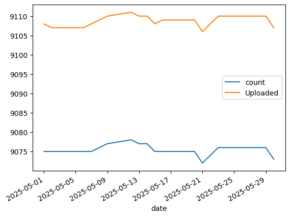
Data Coverage#

As a first step after the risk dataset creation we cross check the asset coverage compared to our raw exposure upload.

upload_stats_df = uploader.get_data_detail_summary()
upload_stats_df.head()

shape: (5, 6)

date	n_assets	min_exposure	max_exposure	mean_exposure	std_exposure
date	i64	f32	f32	f64	f64
2025-05-01	46773	-4.171875	4.28125	0.23534	1.023091
2025-05-02	46766	-4.171875	4.277344	0.235877	1.022765
2025-05-03	46763	-4.171875	4.277344	0.235797	1.022699
2025-05-04	46763	-4.171875	4.277344	0.235795	1.022698
2025-05-05	46766	-4.171875	4.277344	0.236549	1.022354

uploader.get_data().collect()

shape: (14_485_600, 6)

date	asset_id	asset_id_type	factor_group	factor	exposure
date	str	str	str	str	f32
2025-05-01	"IC00009602"	"bayesid"	"market"	"Market"	1.0
2025-05-01	"IC00056DA0"	"bayesid"	"market"	"Market"	1.0
2025-05-01	"IC0007243E"	"bayesid"	"market"	"Market"	1.0
2025-05-01	"IC0007E6E3"	"bayesid"	"market"	"Market"	1.0
2025-05-01	"IC00098715"	"bayesid"	"market"	"Market"	1.0
…	…	…	…	…	…
2025-05-31	"IC8C349DE9"	"bayesid"	"style"	"Dividend"	-0.997559
2025-05-31	"IC8C356E02"	"bayesid"	"style"	"Dividend"	1.438477
2025-05-31	"IC8C36399F"	"bayesid"	"style"	"Dividend"	0.129395
2025-05-31	"IC8C38B75E"	"bayesid"	"style"	"Dividend"	-0.997559
2025-05-31	"IC8C3BF346"	"bayesid"	"style"	"Dividend"	-0.997559

# note that the industry and region hierarchy names tie out with the factor groups we specified above
print(f"Categorical Hierarchies {list(my_risk_dataset.describe().universe_settings_menu.categorical_hierarchies.keys())}")

Categorical Hierarchies ['trbc', 'industry', 'region']

universe_settings = UniverseSettings(dataset=risk_dataset_name)

universe_api = bln.equity.universes.load(universe_settings)
universe_counts = universe_api.counts()

(
    universe_counts
    .join(
        upload_stats_df.select("date", "n_assets").rename({"n_assets": "Uploaded"}),
        on="date",
        how="left",
    )
    .sort("date")
    .to_pandas()
    .set_index("date")
    .plot()
)

<Axes: xlabel='date'>

../_images/a10a5f7baaaca6cb13a2a862ed01a0b89f0f0181be282725578558a93585a60b.png

We can pull some exposures from the new risk dataset to verify.

exposures_api = bln.equity.exposures.load(
    ExposureSettings(
        exposures=[
            ContinuousExposureGroupSettings(hierarchy="market"),
            ContinuousExposureGroupSettings(hierarchy="style", standardize_method="equal_weighted"),
        ],
    )
)

df = exposures_api.get(universe_settings, standardize_universe=None)

df.tail()

shape: (5, 10)

date	bayesid	market.Market	style.Dividend	style.Growth	style.Leverage	style.Momentum	style.Size	style.Value	style.Volatility
date	str	f32	f32	f32	f32	f32	f32	f32	f32
2025-05-31	"ICFFD2AC11"	1.0	-0.128174	-0.615723	2.2734375	1.485352	0.089783	1.848633	1.155273
2025-05-31	"ICFFD5F0F1"	1.0	-0.064941	0.046783	-0.097107	-0.65918	-0.684082	0.282959	-1.556641
2025-05-31	"ICFFE39A3E"	1.0	-0.95752	-0.463867	-1.137695	-0.312256	-1.629883	1.832031	0.979492
2025-05-31	"ICFFE54368"	1.0	-0.95752	-0.869141	0.073914	-1.070312	0.494629	-2.464844	0.652832
2025-05-31	"ICFFEBBB38"	1.0	0.159302	0.405518	0.124146	0.418457	0.080322	0.270508	-1.135742

Model Onboarding

Contents

Model Onboarding#

Exposure Upload#

Data Commit#

Risk Dataset Creation#

Data Coverage#