Custom Dataset From Scratch#

Most of the other tutorials start from a reference risk dataset that Bayesline maintains — bayesline/Bayesline-US-All-1y, Bayesline-Global, etc. You layer your own exposures or filters on top via DerivedRiskDatasetSettings and the engine pulls everything else (master data, prices, calendars, FX) from the reference.

This tutorial covers the other path: building a risk dataset from scratch with no reference. You bring every piece of input yourself. This is the path you take when you have your own house-alpha factors, your own price feed, your own asset master, and you want Bayesline to fit a factor model on top of all of it without any external data dependency.

The mechanism is RootRiskDatasetSettings and the six (+1 optional) upload data types that feed it:

        erDiagram
    idmap ||--o{ market_cap : "asset_id"
    idmap ||--o{ price : "asset_id"
    idmap ||--o{ exposures : "asset_id"
    exchange_rates ||--o{ market_cap : "ccy"
    exchange_rates ||--o{ price : "ccy"

    idmap {
        date start_date
        date end_date
        string from_id_type
        string from_id
        string to_id_type
        string to_id
    }
    market_cap {
        date date PK
        string asset_id PK
        string asset_id_type PK
        string ccy
        float market_cap
        float volume
        float idio_vol
    }
    price {
        date date PK
        string asset_id PK
        string asset_id_type PK
        string ccy PK
        float close
        float return
        bool delisted
    }
    exposures {
        date date PK
        string asset_id PK
        string asset_id_type PK
        string factor_group PK
        string factor PK
        float exposure
    }
    exchange_dates {
        date date PK
        string exchange PK
    }
    exchange_rates {
        date date PK
        string ccy PK
        float fx_rate
    }

One sentence per box:

idmap — which ids refer to the same asset? (ticker → ticker_core, ISIN → ticker, etc.)
market_cap — who is each asset? Slow-changing master data: id, ccy, market cap, volume, idio vol.
price — what did each asset do today? The daily market record: close, daily return, delisted flag.
exposures — what factors does each asset load on? Long format: (date, asset, group, factor, value).
exchange_dates — which days is each exchange closed? Non-trading days, per exchange.
exchange_rates — how do we get to USD? USD-base FX per (date, ccy).

The rest of this tutorial walks one box at a time, simulates a small US universe so everything runs offline, builds a dataset from all six uploads, fits a factor model on top, and checks that the engine recovers the factor returns we simulated.

If you already have a reference dataset that meets your needs, you want Model Onboarding instead — same final shape, derived path.

Imports and client#

We pull in polars for frame construction, numpy for the simulation, and the public bayesline.api.equity settings types we’ll need below.

import datetime as dt

import numpy as np
import polars as pl

from bayesline.apiclient import BayeslineApiClient
from bayesline.api.equity import (
    CategoricalExposureGroupSettings,
    CategoricalFilterSettings,
    ContinuousExposureGroupSettings,
    ExposureSettings,
    FactorRiskModelSettings,
    ModelConstructionSettings,
    RootRiskDatasetSettings,
    UniverseSettings,
)

A real script would connect to your deployment via BayeslineApiClient.new_client(endpoint=..., api_key=...). This tutorial uses the in-process app the docs build provides — every API call below runs end-to-end against the real backend.

bln = BayeslineApiClient.new_client(
    endpoint="https://[ENDPOINT]",
    api_key="[API-KEY]",
)

Simulating a universe#

To keep the tutorial self-contained we generate everything in-notebook: 30 assets on the NYSE, one year of business days, six industries, three style factors, plus a market intercept. Every input frame downstream is derived from the constants in this cell.

The simulation also gives us ground truth: we draw factor returns ourselves, so at the end we can plot the engine’s estimated fret() against what we know the answer should be.

rng = np.random.default_rng(42)

N_ASSETS = 30
INDUSTRIES = ["TECH", "ENERGY", "FINS", "HEALTH", "CONSUMER", "MATERIALS"]
STYLES = ["momentum", "value", "size"]

# 1 year of weekdays ending 2024-12-31. We filter weekends here so the
# simulation doesn't generate prices on Sat/Sun; both weekends and US
# holidays are declared non-trading in the `exchange_dates` upload
# below (the engine's calendar contract).
all_days = pl.date_range(
    dt.date(2024, 1, 2), dt.date(2024, 12, 31), interval="1d", eager=True
).to_list()
dates: list[dt.date] = [d for d in all_days if d.weekday() < 5]
T = len(dates)

# Stable, readable asset ids. In production these would be tickers, ISINs,
# or your house ids — anything as long as it's a stable string.
assets = [f"A{i:04d}" for i in range(N_ASSETS)]

# Per-asset static profile: which industry, what style loadings, what base
# market cap. These are the "who is each asset" attributes that flow into
# market_cap and exposures.
asset_industry = rng.choice(INDUSTRIES, size=N_ASSETS)
asset_style_loadings = rng.standard_normal((N_ASSETS, len(STYLES)))
asset_base_mcap = rng.lognormal(mean=22.0, sigma=1.0, size=N_ASSETS).astype("float32")

print(f"{N_ASSETS} assets × {T} dates ({dates[0]} → {dates[-1]})")
print("industry counts:", dict(zip(*np.unique(asset_industry, return_counts=True))))

30 assets × 261 dates (2024-01-02 → 2024-12-31)
industry counts: {np.str_('CONSUMER'): np.int64(8), np.str_('ENERGY'): np.int64(2), np.str_('FINS'): np.int64(6), np.str_('HEALTH'): np.int64(6), np.str_('MATERIALS'): np.int64(4), np.str_('TECH'): np.int64(4)}

Ground-truth factor returns#

We draw factor returns directly, then build per-asset returns as

\[ r_{i,t} \;=\; f^{\text{market}}_t \;+\; f^{\text{industry}}_{g(i),\,t} \;+\; \sum_k \beta^{\text{style}}_{i,k}\, f^{\text{style}}_{k,t} \;+\; \varepsilon_{i,t}. \]

Industry returns are constrained to a mcap-weighted zero-sum across industries each day — the same constraint we’ll apply in the regression below. That keeps the industry block orthogonal to the market intercept, which is what the engine assumes when zero_sum_constraints={"industry": "mcap_weighted"} is set.

SIGMA_MARKET = 0.010  # ~16% annualized
SIGMA_INDUSTRY = 0.006
SIGMA_STYLE = 0.004
SIGMA_IDIO = 0.015  # ~24% annualized

# Market intercept: one return per day.
f_market = rng.normal(0.0005, SIGMA_MARKET, size=T).astype("float32")

# Industry returns: shape (T, n_industries), then mcap-weighted-zero-summed.
ind_mcap = np.zeros(len(INDUSTRIES), dtype="float32")
for k, g in enumerate(INDUSTRIES):
    ind_mcap[k] = asset_base_mcap[asset_industry == g].sum()
ind_weights = ind_mcap / ind_mcap.sum()

f_industry_raw = rng.normal(0.0, SIGMA_INDUSTRY, size=(T, len(INDUSTRIES))).astype(
    "float32"
)
f_industry = f_industry_raw - (f_industry_raw @ ind_weights)[:, None]
# Sanity: each day's mcap-weighted industry return is ~0.
assert np.allclose((f_industry @ ind_weights), 0.0, atol=1e-6)

# Style returns: shape (T, n_styles).
f_style = rng.normal(0.0, SIGMA_STYLE, size=(T, len(STYLES))).astype("float32")

# Per-asset realized returns: shape (T, N_ASSETS).
ind_idx = np.array([INDUSTRIES.index(g) for g in asset_industry])
r = (
    f_market[:, None]
    + f_industry[:, ind_idx]
    + f_style @ asset_style_loadings.T
    + rng.normal(0.0, SIGMA_IDIO, size=(T, N_ASSETS)).astype("float32")
).astype("float32")

# Stash truth as a tidy frame so the final tie-out chart can join against
# fret(). fret labels factors as `{hierarchy}.{factor}` — `market.market`,
# `industry.TECH`, `style.momentum`, etc. — so we follow the same scheme
# here.
df_truth = pl.concat(
    [
        pl.DataFrame(
            {"date": dates, "factor": "market.market", "true_return": f_market}
        ),
        *[
            pl.DataFrame(
                {
                    "date": dates,
                    "factor": f"industry.{g}",
                    "true_return": f_industry[:, k],
                }
            )
            for k, g in enumerate(INDUSTRIES)
        ],
        *[
            pl.DataFrame(
                {"date": dates, "factor": f"style.{s}", "true_return": f_style[:, k]}
            )
            for k, s in enumerate(STYLES)
        ],
    ]
)
df_truth.head()

shape: (5, 3)

date	factor	true_return
date	str	f32
2024-01-02	"market.market"	-0.009656
2024-01-03	"market.market"	0.003635
2024-01-04	"market.market"	0.008881
2024-01-05	"market.market"	0.020467
2024-01-08	"market.market"	0.029639

Step 1 — `idmap`#

idmap is a temporal table of identifier mappings. It does two jobs in a root dataset:

Resolve foreign ids — ISIN, SEDOL, CUSIP, your house id — onto your canonical master id at query time.
Collapse share classes and cross-listings onto a single master_core id so the engine treats them as the same underlying entity for exposures, market-cap aggregation, and portfolio netting.

Job (2) is what the master vs master_core distinction is for. master is your day-to-day asset id — one row per listing. master_core is the canonical id per entity — one row per underlying company. They are the same id type when every listing is its own entity, and they diverge when one entity has multiple listings.

The textbook example is Alphabet, which trades as two NASDAQ tickers:

GOOGL — Class A, voting shares
GOOG — Class C, non-voting shares

Two listings, one company. To bring both into the dataset and collapse them onto the same entity, you pick one as the core (say GOOG) and upload one projection row per master id:

from_id_type	from_id	to_id_type	to_id
`ticker`	`GOOGL`	`ticker_core`	`GOOG`
`ticker`	`GOOG`	`ticker_core`	`GOOG`

The second row is the identity projection for GOOG — it tells the engine that GOOG itself participates as a master id in your dataset (and is its own core). Without it, GOOG would only be known as the target of GOOGL’s projection, and any market_cap / price / exposures row keyed by GOOG would be silently dropped during dataset construction.

After both rows are in place, GOOGL and GOOG share one set of factor exposures and net to one position when a portfolio is aggregated up — even though they continue to carry independent prices and market caps in the price and market_cap uploads.

A quick warning about using ticker as a master_core type. We use ticker_core in this tutorial because tickers read well, but it’s a poor choice in production: tickers can change for the same company over time. Facebook re-ticker’d from FB to META in 2022, and any dataset using ticker_core as its master_core would split that history into two entities — breaking time-series exposures, returns, and any portfolio that held it across the rename. A good master_core id is permanent across renames, splits, and class consolidations: a vendor permanent id (PERMID, FIGI compid, FactSet entity id) or your house’s stable id. Bayesline’s own datasets use bayesid_core.

Our toy universe has no share-class or cross-listing pairs, so each asset is its own core (the projection is identity). The validity window [0001-01-01, 9999-12-31] keeps each row valid under any as_of_date.

df_idmap = pl.DataFrame(
    {
        "start_date": [dt.date.min] * N_ASSETS,
        "end_date": [dt.date.max] * N_ASSETS,
        "from_id_type": ["ticker"] * N_ASSETS,
        "to_id_type": ["ticker_core"] * N_ASSETS,
        "from_id": assets,
        "to_id": assets,
    }
)
df_idmap.head()

shape: (5, 6)

start_date	end_date	from_id_type	to_id_type	from_id	to_id
date	date	str	str	str	str
0001-01-01	9999-12-31	"ticker"	"ticker_core"	"A0000"	"A0000"
0001-01-01	9999-12-31	"ticker"	"ticker_core"	"A0001"	"A0001"
0001-01-01	9999-12-31	"ticker"	"ticker_core"	"A0002"	"A0002"
0001-01-01	9999-12-31	"ticker"	"ticker_core"	"A0003"	"A0003"
0001-01-01	9999-12-31	"ticker"	"ticker_core"	"A0004"	"A0004"

Step 2 — `market_cap` (entity-level data)#

market_cap answers who is each asset? It carries the asset’s id, functional currency, market cap, daily volume, and an idiosyncratic-vol estimate. Primary key is (date, asset_id, asset_id_type).

Why is this separate from price? Different levels of aggregation. market_cap (and the rest of this row — volume, idio_vol) is an entity-level quantity: one number per company per day. price is a listing-level quantity: one number per traded ticker per currency. Alphabet has two listings — GOOGL and GOOG — that quote at different prices but share a single Alphabet market cap. The convention is to upload one market_cap row per entity, on the master listing (here GOOG, whose master id equals its master_core); repeating it on every listing would double-count when the engine aggregates over the master_core collapse.

In the simulation we build a static per-asset profile, then broadcast across dates with a small random-walk perturbation on market cap so the frame isn’t perfectly constant. volume and idio_vol are constant in this toy — production pipelines fill these from a vendor feed.

# Per-asset static profile (one row per asset).
df_assets = pl.DataFrame(
    {
        "asset_id": assets,
        "base_mcap": asset_base_mcap,
        "volume": rng.uniform(5e5, 5e7, N_ASSETS).astype("float32"),
        "idio_vol": np.full(N_ASSETS, SIGMA_IDIO, dtype="float32"),
    }
)

# Mcap drifts by a small lognormal walk over time so the upload isn't trivially flat.
mcap_walk = np.exp(
    np.cumsum(rng.normal(0.0, 0.005, size=(T, N_ASSETS)), axis=0)
).astype("float32")

# Cross-join dates × assets, then attach the time-varying market cap as a
# column. Polars cross-join order is `(date0, asset0), (date0, asset1), …,
# (date1, asset0), …`, which is exactly the C-order of `mcap_walk[t, i]`.
df_market_cap = (
    pl.DataFrame({"date": dates})
    .join(df_assets, how="cross")
    .with_columns(
        pl.lit("ticker").alias("asset_id_type"),
        pl.lit("USD").alias("ccy"),
        (pl.col("base_mcap") * pl.Series(mcap_walk.reshape(-1)))
        .cast(pl.Float32)
        .alias("market_cap"),
    )
    .select(
        "date", "asset_id", "asset_id_type", "ccy", "market_cap", "volume", "idio_vol"
    )
)
df_market_cap.head()

shape: (5, 7)

date	asset_id	asset_id_type	ccy	market_cap	volume	idio_vol
date	str	str	str	f32	f32	f32
2024-01-02	"A0000"	"ticker"	"USD"	2.9318e9	2.655621e7	0.015
2024-01-02	"A0001"	"ticker"	"USD"	1.3932e9	3.0754266e7	0.015
2024-01-02	"A0002"	"ticker"	"USD"	2.5720e9	2.1954332e7	0.015
2024-01-02	"A0003"	"ticker"	"USD"	8.3242e9	3.8139168e7	0.015
2024-01-02	"A0004"	"ticker"	"USD"	6.36904e8	2.5839e6	0.015

Step 3 — `price` (the daily market record)#

price answers what did each asset do today? It carries close, daily total return, and a delisted flag. Primary key is (date, asset_id, asset_id_type, ccy) — ccy is part of the key so the same asset can carry prices in multiple currencies simultaneously.

We compound the simulated per-asset returns from a base of 100. There’s one wrinkle worth calling out: each asset’s first row must have return = null and serve as the price base. Without that base row the engine has no p[t-1] against which to reconstruct the first realized return. We use a single base row per asset at dates[0] because every asset is alive on day zero in this simulation — a real pipeline with new listings places the base row at each asset’s first appearance.

# Compound returns to a price path starting at 100.
close = np.empty((T, N_ASSETS), dtype="float32")
close[0] = 100.0
close[1:] = 100.0 * np.cumprod(1.0 + r[1:], axis=0)

PRICE_COLS = ["date", "asset_id", "asset_id_type", "ccy", "close", "return", "delisted"]

# Base rows: t=0 for every asset, close=100, return=null (no prior price).
df_price_base = pl.DataFrame({"asset_id": assets}).select(
    pl.lit(dates[0]).alias("date"),
    "asset_id",
    pl.lit("ticker").alias("asset_id_type"),
    pl.lit("USD").alias("ccy"),
    pl.lit(100.0, dtype=pl.Float32).alias("close"),
    pl.lit(None, dtype=pl.Float32).alias("return"),
    pl.lit(False).alias("delisted"),
)

# Realized rows: t=1..T-1, close compounded, return = r[t]. Cross-join
# emits rows in (date, asset) order, matching the C-order reshape of
# close[1:] and r[1:].
df_price_obs = (
    pl.DataFrame({"date": dates[1:]})
    .join(pl.DataFrame({"asset_id": assets}), how="cross")
    .select(
        "date",
        "asset_id",
        pl.lit("ticker").alias("asset_id_type"),
        pl.lit("USD").alias("ccy"),
        pl.Series("close", close[1:].reshape(-1), dtype=pl.Float32),
        pl.Series("return", r[1:].reshape(-1), dtype=pl.Float32),
        pl.lit(False).alias("delisted"),
    )
)

df_price = pl.concat([df_price_base, df_price_obs]).sort("date", "asset_id")
print(
    f"price rows: {df_price.height} (= {N_ASSETS} base + {N_ASSETS * (T - 1)} observed)"
)
df_price.head()

price rows: 7830 (= 30 base + 7800 observed)

shape: (5, 7)

date	asset_id	asset_id_type	ccy	close	return	delisted
date	str	str	str	f32	f32	bool
2024-01-02	"A0000"	"ticker"	"USD"	100.0	null	false
2024-01-02	"A0001"	"ticker"	"USD"	100.0	null	false
2024-01-02	"A0002"	"ticker"	"USD"	100.0	null	false
2024-01-02	"A0003"	"ticker"	"USD"	100.0	null	false
2024-01-02	"A0004"	"ticker"	"USD"	100.0	null	false

Step 4 — `exposures` (long format)#

The exposures upload is long-format with schema (date, asset_id, asset_id_type, factor_group, factor, exposure). Dense vs sparse routing is decided by the engine at dataset-construction time based on which factor groups you declare in dense_factor_groups vs sparse_factor_groups on RootRiskDatasetSettings — there’s no per-row flag.

Conceptually:

Dense factor groups (market, style here) carry a continuous value per asset per day. The engine treats every asset as loading on every factor in a dense group. We upload one row per asset-day-factor.
Sparse factor groups (industry, estimation_universe here) only carry the nonzero loadings — structural zeros are never uploaded. The typical case is one-hot (a pure-play company has a single row per day naming its industry), but multi-row spreads are valid too: a conglomerate with 40% TECH and 60% MATERIALS contributes two rows per day with fractional exposures. The engine routes the sparse block through the path where thin_category_shrinkage actually fires.

We build the three long frames from the static profile and concatenate.

# Per-asset static frames used by the cross joins below. Keeping the
# static profile separate from the date axis is the canonical way to
# build long-format exposures in Polars.
df_asset_industry = pl.DataFrame({"asset_id": assets, "industry": list(asset_industry)})
df_asset_style = pl.DataFrame(
    {
        "asset_id": np.repeat(assets, len(STYLES)),
        "style": STYLES * N_ASSETS,
        "loading": asset_style_loadings.reshape(-1).astype("float32"),
    }
)
df_dates = pl.DataFrame({"date": dates})

# market: dense, every asset loads 1.0 (this is the intercept).
df_exp_market = df_dates.join(
    pl.DataFrame({"asset_id": assets}), how="cross"
).with_columns(
    pl.lit("ticker").alias("asset_id_type"),
    pl.lit("market").alias("factor_group"),
    pl.lit("market").alias("factor"),
    pl.lit(1.0, dtype=pl.Float32).alias("exposure"),
)

# style: dense, one row per (date, asset, style). Loadings are constant
# per asset in this simulation — production pipelines would update them
# daily.
df_exp_style = df_dates.join(df_asset_style, how="cross").select(
    "date",
    "asset_id",
    pl.lit("ticker").alias("asset_id_type"),
    pl.lit("style").alias("factor_group"),
    pl.col("style").alias("factor"),
    pl.col("loading").alias("exposure"),
)

# industry: sparse / categorical. One row per asset-day naming the
# asset's industry.
df_exp_industry = df_dates.join(df_asset_industry, how="cross").select(
    "date",
    "asset_id",
    pl.lit("ticker").alias("asset_id_type"),
    pl.lit("industry").alias("factor_group"),
    pl.col("industry").alias("factor"),
    pl.lit(1.0, dtype=pl.Float32).alias("exposure"),
)

# estimation_universe: sparse, every asset is in our tutorial's estu.
# Production deployments use this group to declare which assets enter
# the regression on each day (e.g. "top 3000 by mcap").
df_exp_estu = df_dates.join(
    pl.DataFrame({"asset_id": assets}), how="cross"
).with_columns(
    pl.lit("ticker").alias("asset_id_type"),
    pl.lit("estimation_universe").alias("factor_group"),
    pl.lit("estimation_universe").alias("factor"),
    pl.lit(1.0, dtype=pl.Float32).alias("exposure"),
)

df_exposures = pl.concat([df_exp_market, df_exp_style, df_exp_industry, df_exp_estu])
print(
    f"exposures rows: {df_exposures.height} "
    f"(market={df_exp_market.height}, style={df_exp_style.height}, "
    f"industry={df_exp_industry.height}, estu={df_exp_estu.height})"
)
df_exposures.head()

exposures rows: 46980 (market=7830, style=23490, industry=7830, estu=7830)

shape: (5, 6)

date	asset_id	asset_id_type	factor_group	factor	exposure
date	str	str	str	str	f32
2024-01-02	"A0000"	"ticker"	"market"	"market"	1.0
2024-01-02	"A0001"	"ticker"	"market"	"market"	1.0
2024-01-02	"A0002"	"ticker"	"market"	"market"	1.0
2024-01-02	"A0003"	"ticker"	"market"	"market"	1.0
2024-01-02	"A0004"	"ticker"	"market"	"market"	1.0

Step 5 — `exchange_dates` (non-trading days)#

exchange_dates carries every non-trading day per exchange — weekends and holidays. The engine doesn’t infer weekends; if a Saturday isn’t in this upload it’s treated as a trading day. The trading calendar for an exchange is (every date in the dataset) ∖ (rows in this upload for that exchange).

We mark both — every Sat/Sun in 2024 plus the US federal holidays for XNYS. A production pipeline would generate this from pandas.tseries.holiday plus a weekday filter, or an exchange-calendar service.

us_holidays_2024 = {
    dt.date(2024, 1, 1),  # New Year
    dt.date(2024, 1, 15),  # MLK
    dt.date(2024, 2, 19),  # Presidents'
    dt.date(2024, 3, 29),  # Good Friday
    dt.date(2024, 5, 27),  # Memorial
    dt.date(2024, 6, 19),  # Juneteenth
    dt.date(2024, 7, 4),  # Independence
    dt.date(2024, 9, 2),  # Labor
    dt.date(2024, 11, 28),  # Thanksgiving
    dt.date(2024, 12, 25),  # Christmas
}
# Weekends + holidays = every non-trading day in range. New Year's Day
# (Jan 1) precedes the Jan-2 start, so only 9 of the 10 listed holidays
# fall in range — recompute the split from the rows so the parts sum to
# the total.
non_trading_days = [d for d in all_days if d.weekday() >= 5 or d in us_holidays_2024]
df_exchange_dates = pl.DataFrame(
    {
        "date": non_trading_days,
        "exchange": ["XNYS"] * len(non_trading_days),
    }
)
n_weekend = sum(1 for d in non_trading_days if d.weekday() >= 5)
n_holiday = len(non_trading_days) - n_weekend
print(
    f"non-trading days: {len(non_trading_days)} "
    f"({n_weekend} weekends + {n_holiday} holidays)"
)
df_exchange_dates.head()

non-trading days: 113 (104 weekends + 9 holidays)

shape: (5, 2)

date	exchange
date	str
2024-01-06	"XNYS"
2024-01-07	"XNYS"
2024-01-13	"XNYS"
2024-01-14	"XNYS"
2024-01-15	"XNYS"

Step 6 — `exchange_rates` (USD-base FX)#

exchange_rates carries USD-base FX per (date, ccy): how many units of ccy equal one USD on that date. So JPY is a large number (≈ 150) and EUR is a small one (≈ 0.93), because one USD buys many yen but less than one euro. Equivalently: to convert a foreign-currency price to USD you divide by fx_rate.

We’re USD-only in this tutorial, so every row has fx_rate = 1.0. A multi-currency pipeline uploads one row per currency per date.

df_exchange_rates = pl.DataFrame(
    {
        "date": dates,
        "ccy": ["USD"] * T,
        "fx_rate": np.ones(T, dtype="float32"),
    }
)
df_exchange_rates.head()

shape: (5, 3)

date	ccy	fx_rate
date	str	f32
2024-01-02	"USD"	1.0
2024-01-03	"USD"	1.0
2024-01-04	"USD"	1.0
2024-01-05	"USD"	1.0
2024-01-08	"USD"	1.0

Upload#

Each of the six frames goes to its own upload data type via the Uploaders API. create_or_replace_dataset(name) creates the upload dataset (or wipes and recreates if it already exists); fast_commit(df, mode="overwrite") stages and commits in one shot. Every frame is built complete in-memory, so each upload is a single "overwrite" commit.

def upload(data_type: str, name: str, df: pl.DataFrame) -> None:
    uploader = bln.equity.uploaders.get_data_type(data_type)
    ds = uploader.create_or_replace_dataset(name)
    ds.fast_commit(df, mode="overwrite")
    print(f"  {data_type:15s} → {name:28s} ({df.height:>7,} rows)")


upload("idmap", "tutorial-idmap", df_idmap)
upload("market_cap", "tutorial-market-cap", df_market_cap)
upload("price", "tutorial-price", df_price)
upload("exposures", "tutorial-exposures", df_exposures)
upload("exchange_dates", "tutorial-exchange-dates", df_exchange_dates)
upload("exchange_rates", "tutorial-exchange-rates", df_exchange_rates)

  idmap           → tutorial-idmap               (     30 rows)

  market_cap      → tutorial-market-cap          (  7,830 rows)

  price           → tutorial-price               (  7,830 rows)

  exposures       → tutorial-exposures           ( 46,980 rows)

  exchange_dates  → tutorial-exchange-dates      (    113 rows)

  exchange_rates  → tutorial-exchange-rates      (    261 rows)

Create the root dataset#

RootRiskDatasetSettings ties the six uploads into a single risk dataset that the rest of the API targets.

Source references. Each *_source= parameter is the name of an upload dataset you created above. The engine resolves them lazily — no data is actually read here.

dense_factor_groups vs sparse_factor_groups. These two dicts decide which regression block the engine routes each factor group through:

Dense — continuous loading per asset per factor (market, style). Every asset loads on every factor in the group.
Sparse — only the nonzero loadings are uploaded (industry, estimation_universe). One-hot membership is the common case, but multi-row spreads are valid: a conglomerate with partial loadings across several industries contributes one row per nonzero entry. The sparse block is also where thin_category_shrinkage fires when the model runs (Step 8).

The dict value — None vs a hierarchy upload source. Each entry pairs a factor-group name with an optional factor hierarchy: a tree that organises the group’s leaves into parent buckets so reports can roll up (GICS sub-industry → industry → sector, value sub-styles → value, etc.). The value is either:

the name of a hierarchy upload dataset you committed alongside the other six (a separate recipe covers this), or
None, which tells the engine to synthesise a flat one-level hierarchy on the fly: each factor in the group becomes its own leaf with no parent, no roll-up structure.

None is the right choice for market and estimation_universe (one factor each — nothing to roll up) and a perfectly fine starting point for style and industry if you don’t have a tree yet. You can replace None with a hierarchy source later without touching any of the six base uploads.

as_of_date snapshots the idmap — only rows whose start_date <= as_of_date are retained when the dataset’s IdMapper is built. Use the most recent date the idmap is authoritative for.

master_id_type / master_id_core_type must match the from_id_type / to_id_type of the master-to-core projection rows in your idmap upload (Step 1).

settings = RootRiskDatasetSettings(
    market_cap_source="tutorial-market-cap",
    price_source="tutorial-price",
    exposures_source="tutorial-exposures",
    exchange_dates_source="tutorial-exchange-dates",
    exchange_rates_source="tutorial-exchange-rates",
    idmap_source="tutorial-idmap",
    dense_factor_groups={"market": None, "style": None},
    sparse_factor_groups={"industry": None, "estimation_universe": None},
    master_id_type="ticker",
    master_id_core_type="ticker_core",
    as_of_date=dates[-1],
)

bln.equity.riskdatasets.delete_dataset_if_exists("tutorial-custom")
dataset = bln.equity.riskdatasets.create_dataset("tutorial-custom", settings)
props = dataset.describe()
print("id types:               ", props.universe_settings_menu.id_types)
print(
    "exchanges:              ",
    props.universe_settings_menu.calendar_settings_menu.exchanges,
)
print(
    "categorical hierarchies:",
    list(props.universe_settings_menu.categorical_hierarchies.keys()),
)
print(
    "continuous hierarchies: ",
    list(props.exposure_settings_menu.continuous_hierarchies.keys()),
)

id types:                ['ticker', 'ticker_core']
exchanges:               ['XNYS']
categorical hierarchies: ['industry', 'estimation_universe']
continuous hierarchies:  ['market', 'style']

Fit a factor model#

FactorRiskModelSettings declares one exposure group per factor block we uploaded. We build the settings dataset-agnostic, then bind them to our new dataset at load time via .with_dataset("tutorial-custom") — the same pattern the other tutorials use.

zero_sum_constraints={"industry": "mcap_weighted"} matches the constraint we applied in the ground-truth simulation, so the engine estimates industry returns in the same gauge.

thin_category_shrinkage={"industry": 10.0} shrinks any industry whose mcap-weighted effective sample size falls below N_min = 10 toward zero — a guard against thin-industry blow-ups. With six industries and 30 assets we’re nowhere near that threshold here, but setting it makes the configuration realistic.

riskmodel_settings = FactorRiskModelSettings(
    universe=UniverseSettings(id_type="ticker"),
    exposures=ExposureSettings(
        exposures=[
            ContinuousExposureGroupSettings(hierarchy="market"),
            CategoricalExposureGroupSettings(hierarchy="industry"),
            ContinuousExposureGroupSettings(hierarchy="style"),
        ]
    ),
    modelconstruction=ModelConstructionSettings(
        estimation_universe=UniverseSettings(
            id_type="ticker",
            categorical_filters=[
                CategoricalFilterSettings(hierarchy="estimation_universe")
            ],
        ),
        zero_sum_constraints={"industry": "mcap_weighted"},
        thin_category_shrinkage={"industry": 10.0},
        return_clip_bounds=(None, None),
    ),
)

model = bln.equity.riskmodels.load(
    riskmodel_settings.with_dataset("tutorial-custom")
).get_model()
df_fret = model.fret()
print("fret shape:", df_fret.shape)
print("factors:   ", {k: len(v) for k, v in model.factors().items()})
df_fret.head()

fret shape: (252, 11)

factors:    {'industry': 6, 'market': 1, 'style': 3}

shape: (5, 11)

date	industry.CONSUMER	industry.ENERGY	industry.FINS	industry.HEALTH	industry.MATERIALS	industry.TECH	market.market	style.momentum	style.size	style.value
date	f32	f32	f32	f32	f32	f32	f32	f32	f32	f32
2024-01-02	0.0	0.0	0.0	0.0	0.0	0.0	0.0	0.0	0.0	0.0
2024-01-03	-0.001508	-0.000547	0.002913	-0.004646	0.00041	0.002329	0.007626	0.00291	-0.006499	0.004172
2024-01-04	0.005483	0.002196	0.002705	-0.010029	-0.003685	-0.000647	0.0086	0.002396	0.001811	-0.00352
2024-01-05	-0.005219	0.000634	0.000258	0.008118	0.001262	-0.000469	0.02151	-0.001198	0.016389	-0.007198
2024-01-08	-0.003841	-0.001597	0.00307	0.000216	0.000478	0.001505	0.025358	-0.009139	-0.0055	-0.002657

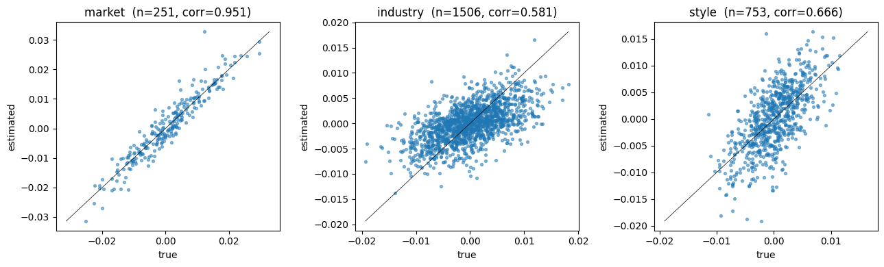
Sanity check: did the engine recover what we simulated?#

Because we generated the factor returns ourselves we know what fret() should look like. Join the estimated returns against df_truth and plot estimated vs true per factor. The points should hug a 45° line — not exactly (idio noise plus regression-weighting choices add scatter), but tightly enough that the dataset is clearly wired correctly.

import matplotlib.pyplot as plt

# fret returns 0.0 on edge dates where the regression can't run (no prior
# price). Drop those rows so the scatter only contains real comparisons.
nonzero_dates = (
    df_fret.unpivot(index="date", variable_name="factor", value_name="estimated")
    .group_by("date")
    .agg(pl.col("estimated").abs().sum().alias("absum"))
    .filter(pl.col("absum") > 0)
    .select("date")
)

df_compare = (
    df_fret.unpivot(index="date", variable_name="factor", value_name="estimated")
    .join(nonzero_dates, on="date", how="inner")
    .join(df_truth, on=("date", "factor"), how="inner")
)
print(f"df_compare rows: {df_compare.height} (dates kept: {nonzero_dates.height})")

groups = ["market", "industry", "style"]
fig, axes = plt.subplots(1, len(groups), figsize=(13, 4))
for ax, g in zip(axes, groups):
    sub = df_compare.filter(pl.col("factor").str.starts_with(g + "."))
    x = sub["true_return"].to_numpy()
    y = sub["estimated"].to_numpy()
    ax.scatter(x, y, s=8, alpha=0.5)
    if x.size:
        lo = float(min(x.min(), y.min()))
        hi = float(max(x.max(), y.max()))
        ax.plot([lo, hi], [lo, hi], color="black", linewidth=0.5)
        corr = float(np.corrcoef(x, y)[0, 1])
        ax.set_title(f"{g}  (n={x.size}, corr={corr:.3f})")
        print(f"{g:8s}  n={x.size:5d}  corr={corr:+.3f}")
    else:
        ax.set_title(f"{g} (no rows)")
    ax.set_xlabel("true")
    ax.set_ylabel("estimated")
fig.tight_layout()
plt.show()

df_compare rows: 2510 (dates kept: 251)
market    n=  251  corr=+0.951
industry  n= 1506  corr=+0.581
style     n=  753  corr=+0.666

../_images/301638e1e812fc25b0e4a110e9f220b6b080bd1d51c0f4919012deda455fd652.png

Out of scope (and where to look next)#

A few capabilities of RootRiskDatasetSettings we deliberately skipped to keep this tutorial focused:

series_source — optional seventh upload of scalar time series (risk-free rate, region-aggregate returns, etc.). Pass series_source="..." on RootRiskDatasetSettings after uploading a frame with (date, series, value).
Uploaded hierarchies — both dense_factor_groups and sparse_factor_groups accept an upload source name in place of None to load a custom factor hierarchy (e.g. sector → industry → sub-industry trees). The default None gives a flat one-level hierarchy, which is what we used.
Catch-up / incremental uploads — see Exposure Catch-up Upload for the pattern of appending new dates to an existing upload dataset.
Building a derived dataset on top of this one — once tutorial-custom exists, you can pass reference_dataset= "tutorial-custom" on DerivedRiskDatasetSettings to layer additional exposures / filters / hierarchies. See Model Onboarding and Risk Datasets.

Custom Dataset From Scratch

Contents